Top 7 Linear Regression Assumptions You Must Know

The theory of linear regression is based on certain statistical assumptions. It is crucial to check these regression assumptions before modeling the data using the linear regression approach. In this blog post, we describe the top 7 assumptions and you should check in DataPandit before analyzing your data using linear regression. Let’s take a look at these assumptions one by one.

#1 There is a Linear Model

The constant terms in a linear model are called parameters whereas the independent variable terms are called predictors for the model. A model is called linear when its parameters are linear. However, it is not necessary to have linear predictors to have a linear model. 

To understand the concept, let’s see how a general a linear model can be written? The answer is as follows:

Response = constant + parameter * predictor + … + parameter * predictor
Or

Y = b _o + b₁X₁ + b₂X₂ + … + b_kX_k

In the above example, it is possible to obtain various curves by transforming the predictor variables (Xs)  using power transformation, logarithmic transformation, square root transformation, inverse transformation, etc. However, the parameter must remain linear always. For example, the following equation represents a linear model because the parameters ( b _o,b_1, and b₂) are linear and only X₁ is raised to the power of 2.

Y = b _o + b₁X₁ + b₂X₁²

In DataPandit the algorithm automatically picks up the linear model when you try to build a linear or a multiple linear regression relationship. Hence you need not check this assumption separately.

#2 There is no multicollinearity

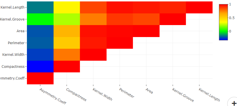
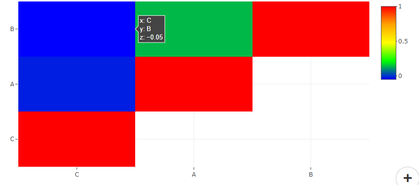
If the predictor variables are correlated among themselves, then the data is said to have a multicollinearity problem.  In other words, if the independent variable columns in your data set are correlated with each other, then there exists multicollinearity within your data. In DataPandit we use Pearson’s Correlation Coefficient to measure the multicollinearity within data. The assumption of no multicollinearity in the data can be easily visualized with the help of the collinearity matrix. 

#3 Homoscedasticity of Residuals or Equal Variances

The linear regression model assumes that there will be always some random error in every measurement. In other words, no two measurements are going to be exactly equal to each other. The constant parameter (b _o ) in the linear regression model represents this random error. However linear regression model does not account for systematic errors which may occur during a process. 

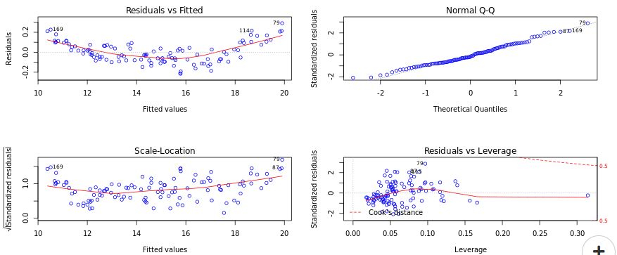
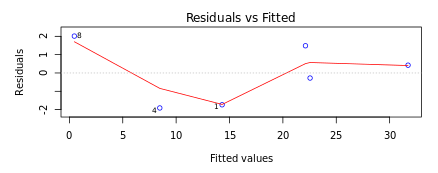
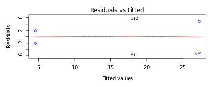
Systematic error is an error with a non-zero mean. In other words, the effect of the systematic error is not reduced when the observations are averaged. For example, loosening of upper and lower punches during the tablet compression process results in lower tablet hardness over a period of time. The absence of such an error can be determined by looking at the Residuals versus fitted values plot in DataPandit. In presence of systematic error, the residuals Vs Fitted values plot will look like Figure 3.

If the Residuals are equally distributed on both sides of the trend line in the residual versus fitted values plot as in Figure 4, then it means there is an absence of systematic error. The idea is that equally distributed residuals or equally distributed variances will average out themselves to zero. Therefore, one can safely assume that measurements only have a random error that can be accounted for by the linear model and there is the absence of systematic error. 

#4 Normality of Residuals

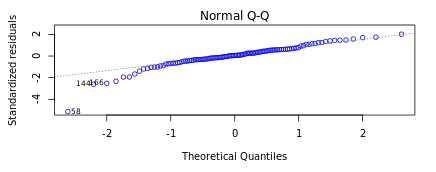
It is important to confirm the normality of residuals for reaffirming the absence of systematic errors as stated above.  It is assumed that if the residuals are normally distributed they are unlikely to have an external influence (systematic error) that will cause them to increase or decrease consistently over a period of time. In DataPandit you can check the assumption for normality of residuals by looking at the Normal Q-Q plot. 

Figure 5 and Figure 6 demonstrate the case when the assumption of normality is not met and the case when the assumption of normality is met respectively.

#5 Number of observations > number of predictors

For a minimum viable model,

Number of observations= Number of Predictors + 1

However greater the number of observations better the model performance. Therefore, to build a linear regression model you must have more observations than the number of independent variables (predictors)  in the data set.

For example, if you are interested in predicting the density based on mass and volume, then you must have data from at least three observations because in this case, you have two predictors namely, mass and volume. 

#6 Each observation is unique

It is also important to ensure that each observation is independent of the other observation.  Meaning each observation in the data set should be recorded/measured separately on a unique occurrence of the event that caused the observation. 

For example, if you want to include two observations to measure the density of a liquid with 2 Kg mass and 2 l volume, then you must perform the experiment twice to measure the density for the two independent observations. Such observations are called replicates of each other. It would be wrong to use same measurement for both observations, as you will disregard the random error.

#7 Predictors are distributed Normally

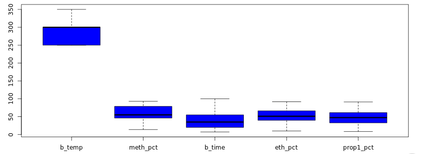
This assumption ensures that you have evenly distributed observations for the range of each predictor. For example, if you want to model the density of a liquid as a function of temperature, then it will make sense to measure the density at different temperature levels within your predefined temperature range. However, if you make more measurements at lower temperatures than at higher temperatures then your model may perform poorly in predicting density at high temperatures. To avoid this problem it will make sense to take a look at the boxplot for checking the normality of predictors. Read this article to know how boxplots can be used to evaluate the normality of variables. For example, in Figure 7, all predictors except ‘b-temp’ are normally distributed.

Closing

So, this was all about assumptions for linear regression. I hope that this information will help you to better prepare yourself for your next linear regression model. 

Need multivariate data analysis software? Apply here to obtain free access to our analytics solutions for research and training purposes!