Introduction to linear regression
Whenever you come across a few variables that seem to be dependent on each other, you might want to explore the linear regression relationship between the variables. linear regression relationship can help you assess:
- The strength of the relationship between the variables
- Possibility of using predictive analytics to measure future outcomes
This article will discuss how linear regression can help you with examples.
Advantages of linear regression
Establishing the linear relationship can be incredibly advantageous if measuring the response variables is either time-consuming or too expensive. In such a scenario, linear regression can help you make soft savings by reducing the consumption of resources.
Linear regression can also provide scientific evidence for establishing a relationship between cause and effect. Therefore the method is helpful in submitting evidence to the regulatory agencies to justify your process controls. In the life-science industry, linear regression can be used as a scientific rationale in the quality by design approach.
Types of linear regression
There are three major types of linear regression as below:
- Simple linear regression: Useful when there is one independent variable and one dependent variable
- Multiple linear regression: Useful when there are multiple independent variables and one dependent variable
Both types of linear regression methods mentioned above need to meet assumptions for Linear regression. You can find these assumptions in our previous article here.
This article will see one example of simple linear regression and one example of multiple linear regression.
Simple linear regression
To understand how to model the relationship between one independent variable and one dependent variable, let’s take the simple example of the BMI dataset. We will explore if there is any relationship between the height and weight of the individuals. Therefore, our Null hypothesis is that ‘There is no relationship between weight and height of the individuals’.
Step I
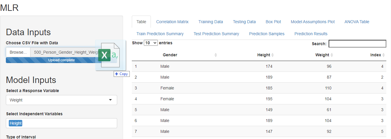
Let’s start by Importing the data. To do this drag and drop your data in the Data Input fields. You can also browse to upload data from your computer.
DataPandit divides your data into train set and test set using default settings where (~59%) of your data gets randomly selected in the train set and the remaining goes into the test set. You have the option to change these settings in the sidebar layout. If your data is small you may want to increase the value higher than 0.59 to include more samples in your train set.
Step II
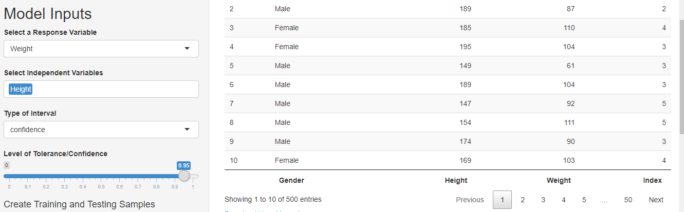
The next step is to give model inputs. Select the dependent variable as the response variable and the independent variable as the predictors. I wanted to use weight as a dependent variable and height as an independent variable hence I made the selections as shown in the figure below.
Step III
Next refer to articles for Pearson’s correlations matrix, box-plots, and models assumptions plot for pre-modeling data analysis. In this case, Pearson’s correlation matrix for two variables won’t display as it is designed for more than two variables. However, if you still wish to see it you can select the height and weight both as independent variables and it will display. After you are done, just remove weight from the independent variables to proceed further.
Step IV
The ANOVA table displays automatically as soon as you select the variables for the model. Hence, after the selection of variables you may simply check the ANOVA table by going to the ANOVA Table tab as shown below:

The p-value for Height in the above ANOVA table is greater than 0.05 which indicates that there are no significant differences in weights of individuals with different heights. Therefore, we fail to reject the null hypothesis. The R squared value and Adjusted R Squared value are also close to zero indicating that the model may not have a high prediction accuracy. The small F- statistic also supports the decision to reject the null hypothesis.
Step V
If you have evidence of a significant relationship between the two variables, you can proceed with train set predictions and test set predictions. The picture below shows the train set predictions for the present case. You can consider this as a model validation step where you evaluating the accuracy of predictions. You can select confidence intervals or prediction intervals in the sidebar layout to understand the range in which future predictions may lie. If you are happy with the train and test predictions you can save your model using the ‘save file’’ option in the sidebar layout.

Step VI
It is the final step in which you use the model for future prediction. In this step you need to upload the saved file using the Upload Model option in the sidebar layout. Then you need to add the data of predictors for which you want to predict the response. In this case, you need to upload the CSV file with the data for the model to predict weights. While uploading the data to make predictions for unknown weights, please ensure that you don’t have the weights column in your data.

Select the response name as Weight and the predictions will populate along with upper and lower limits under the ‘Prediction Results’ tab.

Multiple linear regression
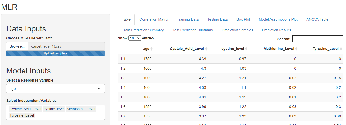
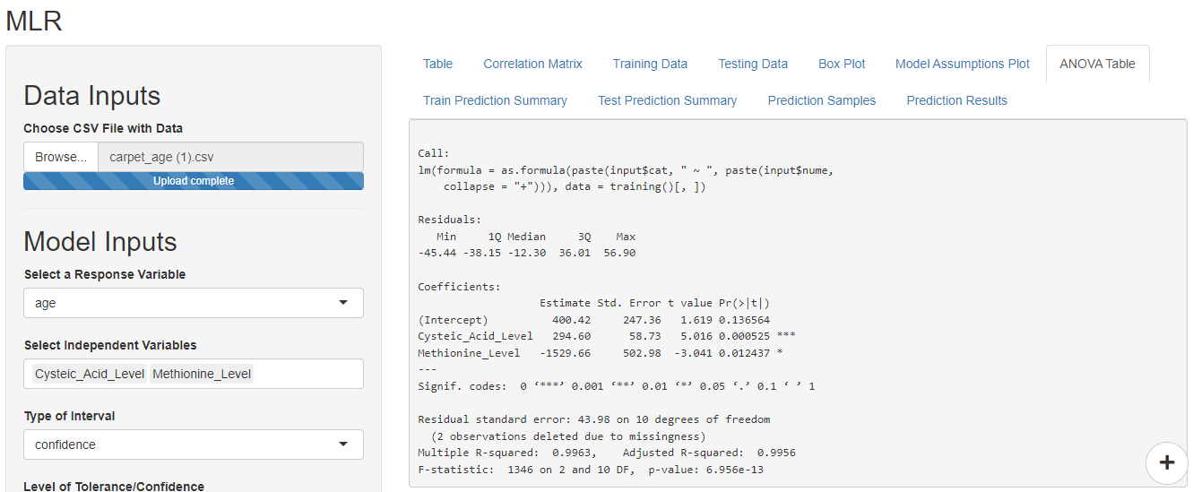
The steps for multiple regression are the same as that of Simple linear regression except that you can choose multiple variables as independent variables. Let’s take an example of detection of the age of carpet based on Chemical levels. The data contains the Age of 23 Old Carpet and Wool samples, along with corresponding levels of chemicals such as Cysteic Acid, Cystine, Methionine, and Tyrosine.
Step I
Same as simple linear regression.
Step II
In this case, we wish to predict the age of the carpet hence, select age as the response variable. Select all other factors as independent variables.
Step III
Same as simple linear regression.
Step IV
The cystine level and tyrosine level do not have a significant p-value hence they can be eliminated from the selected independent variables to improve the model.
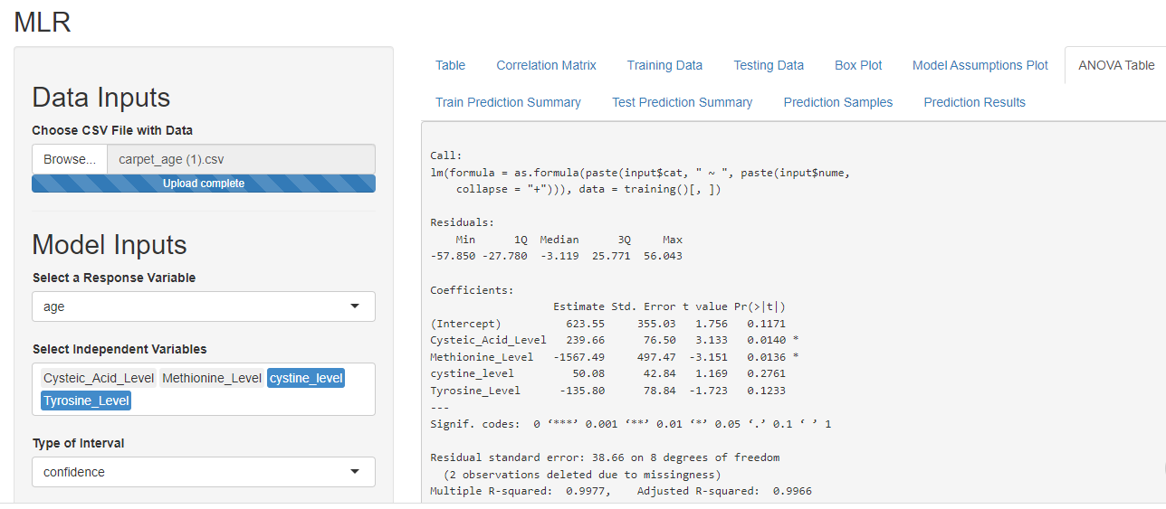
The Anova table automatically updates as soon as you make changes in the ‘Model Inputs’. Based on the p-value, F-statistic, multiple R-square and adjusted R square the model shows a good promise for making future predictions.
Step V
Same as simple linear regression.
Step VI
Same as simple linear regression.
Conclusion
Building linear regression models with DataPandit is a breeze. All you need is well-organized data with a strong scientific backing. Because correlation does not imply causation!
Need multivariate data analysis software? Apply here to obtain free access to our analytics solutions for research and training purposes!